Training a PyKAN Neural Network for Regression and Prediction

Overview

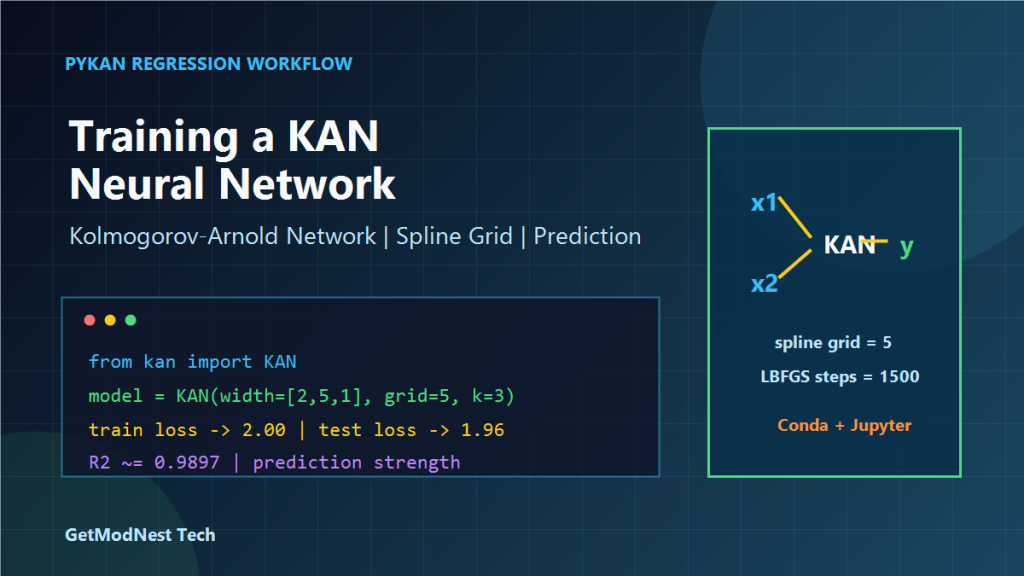
This article documents a practical PyKAN workflow for training a Kolmogorov-Arnold Network on a small regression problem. The notes cover dataset construction, KAN model creation, training, result analysis, prediction usage, Windows environment setup, and Jupyter Notebook execution.

The overall workflow is:

prepare numeric data -> build PyKAN model -> train regression model -> analyze loss and R2 -> run prediction -> use model in Jupyter

KAN, or Kolmogorov-Arnold Network, is a neural network architecture that uses learnable spline functions. Compared with a traditional MLP, a KAN model can sometimes provide better interpretability because nonlinear transformations are represented on edges by spline-like functions.

Goal

The goal of this experiment was to train a PyKAN model on two input variables and predict one continuous target value.

The problem can be written as:

y = f(x1, x2)

This is a regression task. The model receives two numeric inputs and outputs one predicted numeric value.

Dataset Construction

The recorded dataset contains two input features:

x1
x2

and one output target:

y = f(x1, x2)

The training and test data can be generated with NumPy or prepared from a real numeric dataset.

Example structure:

input:  x1, x2
target: y
problem type: regression

A typical PyKAN dataset dictionary contains:

dataset = {
    "train_input": train_input,
    "train_label": train_label,
    "test_input": test_input,
    "test_label": test_label,
}

The input tensors should have shape similar to:

[number_of_samples, 2]

and the labels should have shape similar to:

[number_of_samples, 1]

Create a KAN Model

A basic KAN model can be created with:

from kan import KAN

model = KAN(
    width=[2, 5, 1],
    grid=5,
    k=3,
)

The meaning of these parameters is:

width=[2, 5, 1]   two input nodes, five hidden units, one output node
grid=5            spline grid size
k=3               spline order

In this setup:

input dimension: 2
hidden layer: 5 KAN units
output dimension: 1
task type: regression

This is a relatively small KAN model, suitable for simple regression experiments and quick tests.

Train the KAN Model

The model was trained for around 1500 epochs in the recorded experiment.

Example training call:

results = model.train(
    dataset,
    opt="LBFGS",
    steps=1500,
    lamb=4.0e-2,
)

The regularization term was approximately:

regularization: about 4.0e-2

During training, both training loss and test loss should be monitored.

Recorded trend:

train loss: about 2.50 -> 2.05 -> 2.00 range
test loss:  about 2.88 -> 2.10 -> 1.96 range

The exact values may vary depending on dataset generation, random seed, PyKAN version, and model configuration.

Training Observations

The training logs showed that the loss decreased over time.

Important observations:

training loss decreased gradually
test loss also decreased
regularization helped control spline complexity
the final test loss was around 1.96 in the recorded run

The notes also mention that the spline functions became more stable after training. This is expected because KAN learns nonlinear functions on network edges.

Result Analysis

After training, the model result can be evaluated using regression metrics and plots.

Recorded result examples:

R2: about 0.98973
relative error: about 0.64%
predicted values were close to actual values

Typical analysis steps include:

compare predicted values with actual values
plot prediction vs actual values
plot residual errors
check whether the model overfits
check whether spline functions are too complex

The notes also highlight several important factors:

a/R may be the most important feature, around 68.76% influence
another feature may contribute around 11.24%
the model is relatively stable but not always fully interpretable

The exact feature influence depends on the dataset and interpretation method.

Prediction Usage

After the model is trained, it can be used to predict new samples.

Example idea:

predict_strength(a_over_r, jingt)

A prediction function can receive input features and return a predicted strength value.

Conceptually:

input:  a/R and Jingt value
output: predicted strength

Example usage:

strength = predict_strength(0.2, "jingt")
print(strength)

The notes mention example predicted strength values such as:

1625.47
1630.29

These values are examples from the recorded experiment and should be interpreted based on the original dataset units.

Windows Environment Setup for PyKAN

On Windows, it is recommended to create a separate Conda environment for PyKAN.

Create the environment:

conda create -n pykan-env python=3.10.19

Activate it:

conda activate pykan-env

Download or place the PyKAN project into a working directory, for example:

D:\CODE\pykan

Install dependencies:

pip install -r requirements.txt

If the package needs to be installed in editable mode:

pip install -e . --force-reinstall

If imports fail, check whether the package directory is correctly installed and whether the environment is activated.

Verify the PyKAN Import

Test the import in Python:

from kan import KAN

If the import succeeds, the PyKAN package is available in the current environment.

If it fails, check:

current Conda environment
package installation path
whether pip installed into the correct Python environment
whether there are conflicting package names

Jupyter Notebook Setup

To use PyKAN inside Jupyter Notebook, install an IPython kernel for the Conda environment.

Example command:

python -m ipykernel install --user --name=pykan-env --display-name "Python (pykan-env)"

Then start Jupyter Notebook:

jupyter notebook

If the browser does not open automatically, copy the URL shown in the terminal. It may look like:

http://localhost:8888/tree?token=...

If you want to start Jupyter without opening the browser automatically:

jupyter notebook --no-browser

Then manually open:

http://localhost:8888

In the notebook, select the Python (pykan-env) kernel.

Minimal Jupyter Test

Inside Jupyter Notebook, run:

import torch
from kan import KAN

model = KAN(width=[2, 5, 1], grid=5, k=3)
print(model)

If this runs successfully, the environment and PyKAN installation are working.

Common Problems

PyKAN Cannot Be Imported

Check whether the correct Conda environment is active:

conda activate pykan-env

Then reinstall the package:

pip install -e . --force-reinstall

Also check whether the current Python executable belongs to the same environment.

Jupyter Does Not Show the Environment Kernel

Install the kernel again:

python -m ipykernel install --user --name=pykan-env --display-name "Python (pykan-env)"

Restart Jupyter Notebook and select the new kernel.

Training Loss Does Not Decrease

Possible reasons include:

input data is not normalized
target values have large scale differences
model width is too small
regularization is too strong
the learning optimizer or training steps are not suitable
data contains noise or outliers

Try normalizing the input features and target values before training.

Model Overfits

If training loss is low but test loss remains high, try:

increase regularization
reduce model width
reduce spline grid size
use more training data
check for data leakage

Predictions Are Unstable

Check:

feature scaling
input order
tensor shape
training data coverage
random seed
model save and load process

For regression tasks, predictions outside the training data range may be unreliable.

Practical Notes

Important lessons from the experiment:

KAN can fit nonlinear regression relationships
training and test loss should both be monitored
grid size and regularization affect spline complexity
feature scaling is important for stable training
Jupyter kernel configuration is often the source of environment confusion
prediction functions should validate input ranges

When using PyKAN for real projects, always compare predictions with a baseline model such as linear regression, random forest, XGBoost, or a small MLP.

Final Conclusion

This PyKAN experiment demonstrates a complete workflow for regression training and prediction.

The core process is:

prepare x1 and x2 input features
build a KAN model with width=[2, 5, 1]
train the model for regression
monitor train loss and test loss
evaluate R2 and prediction error
use the trained model for prediction
run the workflow inside a Conda and Jupyter environment

KAN is useful for exploring nonlinear regression problems and inspecting learned spline behavior. However, for practical prediction tasks, it should still be validated carefully with test data, residual analysis, and comparison against simpler baseline models.

Need Help with a Similar Problem or Project?

This note is based on a real troubleshooting, configuration, or development workflow. If you need help with databases, Linux servers, web applications, desktop software, iOS and Android apps, automation scripts, deployment, WordPress, or AI development environments, GetModNest can provide practical technical support, troubleshooting, and development assistance.

Email: info@getmodnest.com